You can find a slide presentation here.
INTRODUCCTION
You are a junior data analyst working in the marketing analyst team at Cyclistic, a bike-share company in Chicago. The director of marketing believes the company's future success depends on maximizing the number of annual memberships. Therefore, your team wants to understand how casual riders and annual members use Cyclistic bikes differently. From these insights, your team will design a new marketing strategy to convert casual riders into annual members. But first, Cyclistic executives must approve your recommendations, so they must be backed up with compelling data insights and professional data visualizations.
SCENARIO
You are a junior data analyst working in the marketing analyst team at Cyclistic, a bike-share company in Chicago. The director of marketing believes the company's future success depends on maximizing the number of annual memberships. Therefore, your team wants to understand how casual riders and annual members use Cyclistic bikes differently. From these insights, your team will design a new marketing strategy to convert casual riders into annual members.
Characters and Teams
Cyclistic: A bike-sharing program that includes 5,800 bicycles and 600 stations. Cyclistic stands out for also offering recumbent bikes, hand tricycles, and cargo bikes that provide a more inclusive bike-sharing experience for people with disabilities and cyclists who cannot use a standard two-wheeled bicycle. Most cyclists choose traditional bikes, while around 8% of cyclists use the assisted options. Cyclistic users are more likely to ride for recreation, but about 30% use the bikes for commuting to work each day.
Lily Moreno: The Director of Marketing and your manager. Moreno is responsible for developing campaigns and initiatives to promote the bike-sharing program. Campaigns may include email, social media, and other channels.
Cyclistic's Marketing Data Analytics Team: A team of data analysts responsible for collecting, analyzing, and reporting data that helps drive Cyclistic's marketing strategy. You joined this team six months ago, and you have been dedicated not only to understanding Cyclistic's mission and business goals but also to finding ways to help Cyclistic achieve them from your position as a junior data analyst.
Cyclistic Executive Team: The highly detail-oriented executive team will decide whether to approve the recommended marketing program.
About the Company
In 2016, Cyclistic launched a successful bike-sharing service. Since then, the program has grown to include a fleet of 5,824 geo-referenced bicycles, locked within a network of 692 stations throughout Chicago. The bikes can be unlocked from one station and returned to any other station in the system at any time.
Until now, Cyclistic's marketing strategy has focused on building general brand recognition and attracting broad consumer segments. One of the key approaches that made this possible was the flexibility of their pricing plans: single-ride passes, full-day passes, and annual memberships. Customers who purchase single-ride or full-day passes are called casual riders. Customers who purchase annual memberships are called Cyclistic members.
Cyclistic's financial analysts concluded that annual members are far more profitable than casual riders. While the flexible pricing helps Cyclistic attract more customers, Moreno believes that maximizing the number of annual members will be key to future growth. Rather than creating a marketing campaign aimed at all new customers, Moreno believes there is significant potential to convert casual riders into members. She points out that casual riders are already familiar with Cyclistic's program and have chosen Cyclistic for their mobility needs.
Moreno set a clear goal: to design marketing strategies aimed at converting casual riders into annual members. However, to do so, the marketing analytics team needs a better understanding of how annual members and casual riders differ, why casual riders would purchase a membership, and how digital media might influence their marketing tactics. Moreno and her team are interested in analyzing Cyclistic's historical bike trip data to identify trends.
Questions
Three questions will guide the future marketing program:
- How do annual members and casual riders differ in their use of Cyclistic's bikes?
- Why would casual riders purchase annual memberships from Cyclistic?
- How can Cyclistic use digital media to influence casual riders to become members?
Moreno assigned you the first question to answer: How do annual members and casual riders differ in their use of Cyclistic's bikes?
You will create a report with the following deliverables:
- A clear instruction of the business task
- A description of all data sources used
- Documentation of all data cleaning and manipulations
- A summary of your analysis
- Supporting visualizations and key findings
- The three most important recommendations based on your analysis
This project will follow the steps of the data analysis process: ask, prepare, process, analyze, share, and act.
PREPARE
Historical ride data from Cyclistic will be used to analyze and identify trends. The latest 12 months of Cyclistic ride data can be downloaded here. (Note: The datasets have different datasets are appropriate and will enable the answering of the company's questions. The data has been provided by Motivate International Inc. under this license.) These are public data that can be utilized to explore how different types of customers use Cyclistic bikes. However, it should be noted that, for privacy reasons, the use of personally identifiable information of cyclists is prohibited. This means that connections between pass purchases and credit card numbers cannot be established to determine if casual riders reside within the Cyclistic service area or if they have purchased multiple single-ride passes. The data for the entire year of 2023 was selected to avoid biases associated with partial periods and to ensure that factors such as holidays, seasons, and other seasonal patterns that may influence bicycle usage are taken into account, also meets the ROCCC criteria (Relevant, Original, Complete, Consistent, and Correct), ensuring the quality and reliability of the data for conducting an accurate analysis.
PROCESS
R with will be used for data analysis, statistics, and visualization due to their significant advantages. R is specifically designed for statistical tasks, featuring an extensive ecosystem of packages that enhance its capabilities, such as ggplot2 for visualization and dplyr for data manipulation. The active R community provides abundant resources and support. RStudio serves as an integrated development environment (IDE) that facilitates project organization, includes tools for syntax highlighting and debugging, and supports version control systems like Git. Additionally, RStudio's integration with R Markdown allows for the creation of reproducible documents that combine text, code, and results, making it ideal for reporting. Together, R and RStudio create a powerful combination preferred by analysts and data scientists.
The data for the year comes in 12 separate CSV files, one for each month. Once downloaded, the compare_df_cols_same() function from the janitor package was used to verify that all 12 datasets were suitable for merging.
We start with loading the packages we will use.
library(tidyverse)
library(lubridate)
library(ggplot2)
library(dplyr)
library(janitor)

## Warning: package 'janitor' was built under R version 4.4.3

library(scales)

## Warning: package 'scales' was built under R version 4.4.3

library(viridis)

## Warning: package 'viridis' was built under R version 4.4.3

library(hrbrthemes)

## Warning: package 'hrbrthemes' was built under R version 4.4.3

library(almanac)

## Warning: package 'almanac' was built under R version 4.4.3

library(Cairo)

getwd()

## [1] "D:/Proyecto_R"

setwd("D:/Proyecto_R")
Collect data
Load the datasets and rename
M01_2023 <- read_csv("202301-divvy-tripdata.csv")
M02_2023 <- read_csv("202302-divvy-tripdata.csv")
M03_2023 <- read_csv("202303-divvy-tripdata.csv")
M04_2023 <- read_csv("202304-divvy-tripdata.csv")
M05_2023 <- read_csv("202305-divvy-tripdata.csv")
M06_2023 <- read_csv("202306-divvy-tripdata.csv")
M07_2023 <- read_csv("202307-divvy-tripdata.csv")
M08_2023 <- read_csv("202308-divvy-tripdata.csv")
M09_2023 <- read_csv("202309-divvy-tripdata.csv")
M10_2023 <- read_csv("202310-divvy-tripdata.csv")
M11_2023 <- read_csv("202311-divvy-tripdata.csv")
M12_2023 <- read_csv("202312-divvy-tripdata.csv")
WRANGLE DATA AND COMBINE INTO A SINGLE FILE
Before combining the datasets, it was checked whether the data frames were row-bindable. The function compare_df_cols() was used, which returns TRUE if there are no mismatching rows.
compare_df_cols_same(M01_2023,M02_2023,M03_2023,M04_2023,M05_2023,M06_2023,M07_2023,M08_2023,M09_2023,M10_2023,M11_2023,M12_2023)

## [1] TRUE
All the data was combined into a single data frame, and incongruities were searched for.
annual_data <-bind_rows(M01_2023,M02_2023,M03_2023,M04_2023,M05_2023,M06_2023,M07_2023,M08_2023,M09_2023,M10_2023,M11_2023,M12_2023)
str(annual_data)

## spc_tbl_ [5,719,877 x 13] (S3: spec_tbl_df/tbl_df/tbl/data.frame)
##  $ ride_id           : chr [1:5719877] "F96D5A74A3E41399" "13CB7EB698CEDB88" "BD88A2E670661CE5" "C90792D034FED968" ...
##  $ rideable_type     : chr [1:5719877] "electric_bike" "classic_bike" "electric_bike" "classic_bike" ...
##  $ started_at        : POSIXct[1:5719877], format: "2023-01-21 20:05:42" "2023-01-10 15:37:36" ...
##  $ ended_at          : POSIXct[1:5719877], format: "2023-01-21 20:16:33" "2023-01-10 15:46:05" ...
##  $ start_station_name: chr [1:5719877] "Lincoln Ave & Fullerton Ave" "Kimbark Ave & 53rd St" "Western Ave & Lunt Ave" "Kimbark Ave & 53rd St" ...
##  $ start_station_id  : chr [1:5719877] "TA1309000058" "TA1309000037" "RP-005" "TA1309000037" ...
##  $ end_station_name  : chr [1:5719877] "Hampden Ct & Diversey Ave" "Greenwood Ave & 47th St" "Valli Produce - Evanston Plaza" "Greenwood Ave & 47th St" ...
##  $ end_station_id    : chr [1:5719877] "202480.0" "TA1308000002" "599" "TA1308000002" ...
##  $ start_lat         : num [1:5719877] 41.9 41.8 42 41.8 41.8 ...
##  $ start_lng         : num [1:5719877] -87.6 -87.6 -87.7 -87.6 -87.6 ...
##  $ end_lat           : num [1:5719877] 41.9 41.8 42 41.8 41.8 ...
##  $ end_lng           : num [1:5719877] -87.6 -87.6 -87.7 -87.6 -87.6 ...
##  $ member_casual     : chr [1:5719877] "member" "member" "casual" "member" ...
Columns were renamed to make them understandable.
annual_data <- rename(annual_data, user_type = member_casual)
CLEAN
The duration of each ride in minutes will be calculated and stored in the ride_length column. The difftime function computes the difference between the ended_at and started_at timestamps. Initially, the result is of class difftime, which is not suitable for direct numerical operations.
annual_data$ride_length <- difftime(annual_data$ended_at, annual_data$started_at, units = "mins")
It was verified that the user_type column only had two possible values, and it was checked for duplicates and empty IDs.
unique(annual_data$user_type)

## [1] "member" "casual"

sum(duplicated(annual_data$ride_id))

## [1] 0

sum(is.na(annual_data$ride_id))

## [1] 0

sum(is.na(annual_data$ride_length))

## [1] 0
Columns will be added to list the date, month, day, and year of each ride. This will facilitate the aggregation of ride data by month, day, or year.
annual_data$date <- as.Date(annual_data$started_at) #The default format is yyyy-mm-dd
annual_data$month <- format(as.Date(annual_data$date), "%m")
annual_data$day <- format(as.Date(annual_data$date), "%d")
annual_data$year <- format(as.Date(annual_data$date), "%Y")
annual_data$day_of_week <- format(as.Date(annual_data$date), "%A")
glimpse(annual_data)

## Rows: 5,719,877
## Columns: 19
## $ ride_id            <chr> "F96D5A74A3E41399", "13CB7EB698CEDB88", "BD88A2E670...
## $ rideable_type      <chr> "electric_bike", "classic_bike", "electric_bike", "...
## $ started_at         <dttm> 2023-01-21 20:05:42, 2023-01-10 15:37:36, 2023-01-...
## $ ended_at           <dttm> 2023-01-21 20:16:33, 2023-01-10 15:46:05, 2023-01-...
## $ start_station_name <chr> "Lincoln Ave & Fullerton Ave", "Kimbark Ave & 53rd ...
## $ start_station_id   <chr> "TA1309000058", "TA1309000037", "RP-005", "TA130900...
## $ end_station_name   <chr> "Hampden Ct & Diversey Ave", "Greenwood Ave & 47th ...
## $ end_station_id     <chr> "202480.0", "TA1308000002", "599", "TA1308000002", ...
## $ start_lat          <dbl> 41.92407, 41.79957, 42.00857, 41.79957, 41.79957, 4...
## $ start_lng          <dbl> -87.64628, -87.59475, -87.69048, -87.59475, -87.594...
## $ end_lat            <dbl> 41.93000, 41.80983, 42.03974, 41.80983, 41.80983, 4...
## $ end_lng            <dbl> -87.64000, -87.59938, -87.69941, -87.59938, -87.599...
## $ user_type          <chr> "member", "member", "casual", "member", "member", "...
## $ ride_length        <drtn> 10.850000 mins, 8.483333 mins, 13.233333 mins, 8.7...
## $ date               <date> 2023-01-21, 2023-01-10, 2023-01-02, 2023-01-22, 20...
## $ month              <chr> "01", "01", "01", "01", "01", "01", "01", "01", "01...
## $ day                <chr> "21", "10", "02", "22", "12", "31", "15", "25", "25...
## $ year               <chr> "2023", "2023", "2023", "2023", "2023", "2023", "20...
## $ day_of_week        <chr> "sabado", "martes", "lunes", "domingo", "jueves", "...
The language will be changed to English, and a column will be added for ride length.
annual_data <-  annual_data %>%
  mutate(day_of_week = recode(day_of_week
                              ,"lunes" = "Monday"
                              ,"martes" = "Tuesday"
                              ,"miercoles" = "Wednesday"
                              ,"jueves" = "Thursday"
                              ,"viernes" = "Friday"
                              ,"sabado" = "Saturday"
                              ,"domingo" = "Sunday"))
Use glimpse to inspect the data and verify the type of the ride_length column. It is important to note that the ride_length column is initially of class difftime.
glimpse(annual_data)

## Rows: 5,719,877
## Columns: 19
## $ ride_id            <chr> "F96D5A74A3E41399", "13CB7EB698CEDB88", "BD88A2E670...
## $ rideable_type      <chr> "electric_bike", "classic_bike", "electric_bike", "...
## $ started_at         <dttm> 2023-01-21 20:05:42, 2023-01-10 15:37:36, 2023-01-...
## $ ended_at           <dttm> 2023-01-21 20:16:33, 2023-01-10 15:46:05, 2023-01-...
## $ start_station_name <chr> "Lincoln Ave & Fullerton Ave", "Kimbark Ave & 53rd ...
## $ start_station_id   <chr> "TA1309000058", "TA1309000037", "RP-005", "TA130900...
## $ end_station_name   <chr> "Hampden Ct & Diversey Ave", "Greenwood Ave & 47th ...
## $ end_station_id     <chr> "202480.0", "TA1308000002", "599", "TA1308000002", ...
## $ start_lat          <dbl> 41.92407, 41.79957, 42.00857, 41.79957, 41.79957, 4...
## $ start_lng          <dbl> -87.64628, -87.59475, -87.69048, -87.59475, -87.594...
## $ end_lat            <dbl> 41.93000, 41.80983, 42.03974, 41.80983, 41.80983, 4...
## $ end_lng            <dbl> -87.64000, -87.59938, -87.69941, -87.59938, -87.599...
## $ user_type          <chr> "member", "member", "casual", "member", "member", "...
## $ ride_length        <drtn> 10.850000 mins, 8.483333 mins, 13.233333 mins, 8.7...
## $ date               <date> 2023-01-21, 2023-01-10, 2023-01-02, 2023-01-22, 20...
## $ month              <chr> "01", "01", "01", "01", "01", "01", "01", "01", "01...
## $ day                <chr> "21", "10", "02", "22", "12", "31", "15", "25", "25...
## $ year               <chr> "2023", "2023", "2023", "2023", "2023", "2023", "20...
## $ day_of_week        <chr> "Saturday", "Tuesday", "Monday", "Sunday", "Thursda...
Convert the ride_length column from difftime to a numeric type to enable further numerical operations. This conversion is necessary because difftime objects cannot be directly utilized in mathematical calculations.
annual_data$ride_length <- as.numeric(annual_data$ride_length)

#remove rows from the data frame that have NA values in at least one column
annual_data_v2 <- annual_data[complete.cases(annual_data),]
sum(is.na(annual_data_v2))

## [1] 0

glimpse(annual_data_v2)

## Rows: 4,331,707
## Columns: 19
## $ ride_id            <chr> "F96D5A74A3E41399", "13CB7EB698CEDB88", "BD88A2E670...
## $ rideable_type      <chr> "electric_bike", "classic_bike", "electric_bike", "...
## $ started_at         <dttm> 2023-01-21 20:05:42, 2023-01-10 15:37:36, 2023-01-...
## $ ended_at           <dttm> 2023-01-21 20:16:33, 2023-01-10 15:46:05, 2023-01-...
## $ start_station_name <chr> "Lincoln Ave & Fullerton Ave", "Kimbark Ave & 53rd ...
## $ start_station_id   <chr> "TA1309000058", "TA1309000037", "RP-005", "TA130900...
## $ end_station_name   <chr> "Hampden Ct & Diversey Ave", "Greenwood Ave & 47th ...
## $ end_station_id     <chr> "202480.0", "TA1308000002", "599", "TA1308000002", ...
## $ start_lat          <dbl> 41.92407, 41.79957, 42.00857, 41.79957, 41.79957, 4...
## $ start_lng          <dbl> -87.64628, -87.59475, -87.69048, -87.59475, -87.594...
## $ end_lat            <dbl> 41.93000, 41.80983, 42.03974, 41.80983, 41.80983, 4...
## $ end_lng            <dbl> -87.64000, -87.59938, -87.69941, -87.59938, -87.599...
## $ user_type          <chr> "member", "member", "casual", "member", "member", "...
## $ ride_length        <dbl> 10.850000, 8.483333, 13.233333, 8.766667, 15.316667...
## $ date               <date> 2023-01-21, 2023-01-10, 2023-01-02, 2023-01-22, 20...
## $ month              <chr> "01", "01", "01", "01", "01", "01", "01", "01", "01...
## $ day                <chr> "21", "10", "02", "22", "12", "31", "15", "25", "25...
## $ year               <chr> "2023", "2023", "2023", "2023", "2023", "2023", "20...
## $ day_of_week        <chr> "Saturday", "Tuesday", "Monday", "Sunday", "Thursda...
Verify that all ride lengths are positive and that there are no empty values.
#search for negative values, less than 1 or grater than one day (1440 minutes)
sum((annual_data$ride_length<=0))

## [1] 1269

annual_data_v2 %>%
  filter(ride_length<=0 | ride_length  > 1440)

## # A tibble: 702 x 19
##    ride_id          rideable_type started_at          ended_at
##    <chr>            <chr>         <dttm>              <dttm>
##  1 F4F4A74BF1FB016D classic_bike  2023-01-06 15:59:56 2023-01-07 16:41:17
##  2 3F5B7E5AD8A6FE18 electric_bike 2023-01-17 08:31:49 2023-01-17 08:31:49
##  3 5394CACAFE68B950 electric_bike 2023-01-05 09:10:39 2023-01-05 09:10:39
##  ...

#applying the result
annual_data_v2 <- annual_data_v2 %>%
  filter(!(ride_length<=1 | ride_length  > 1440))

#search for NA values in ride_length column
sum(is.na(annual_data_v2$ride_length))

## [1] 0

glimpse(annual_data_v2)

## Rows: 4,243,193
## Columns: 19

summary(annual_data_v2)

##    ride_id          rideable_type        started_at
##  Length:4243193     Length:4243193     Min.   :2023-01-01 00:02:06.00
##  Class :character   Class :character   1st Qu.:2023-05-20 18:06:14.00
##  Mode  :character   Mode  :character   Median :2023-07-20 18:29:02.00
##                                        Mean   :2023-07-16 01:55:18.68
##                                        3rd Qu.:2023-09-16 19:11:08.00
##                                        Max.   :2023-12-31 23:58:55.00
ANALYSIS
How do annual members and casual riders differ in their use of Cyclistic's bikes? Based on the quartiles, most ride duration fall below 50 minutes. By setting this limit, the focus remains on the most relevant portion of the dataset, avoiding the distortion caused by extreme outliers. This helps to clearly visualize the central distribution of the data without being skewed by a few extreme values.
sum(is.na(annual_data_v2$ride_length))

## [1] 0

Q1 <- quantile(annual_data_v2$ride_length, 0.25, na.rm = TRUE)
Q3 <- quantile(annual_data_v2$ride_length, 0.75, na.rm = TRUE)

IQR_value <- Q3 - Q1

### Definir limites (1.5 veces el IQR)
lower_bound <- Q1 - 1.5 * IQR_value
upper_bound <- Q3 + 1.5 * IQR_value

### Filtrar los valores dentro de estos limites
annual_data_v2 <- annual_data_v2 %>%
 filter(ride_length >= lower_bound & ride_length <= upper_bound)

# Crear el grafico de violin con los datos filtrados
annual_data_v2 %>%
  ggplot(aes(x = user_type, y = ride_length, fill = user_type)) +
  geom_violin(width = .4) +
  geom_boxplot(width = 0.1, color = "black", alpha = 0.2, outlier.shape = NA) +
  scale_fill_manual(values=c("#4DB6AC", "#FFAB40")) +
  theme_ipsum() +
  labs(title = "Ride length distribution by user type ",
  x ="User type",y= "Ride Length (min)", fill = "User type")
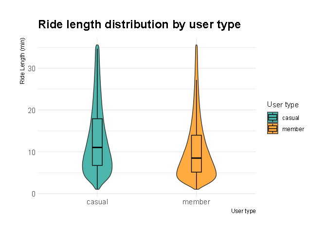 Ride length distribution by user type
Convert numeric month representation to month names
typeof(annual_data_v2$month)

## [1] "character"

annual_data_v2 <-  annual_data_v2 %>%
  mutate(month = recode(month
                              ,"01" = "January"
                              ,"02" = "February"
                              ,"03" = "March"
                              ,"04" = "April"
                              ,"05" = "May"
                              ,"06" = "June"
                              ,"07" = "July"
                              ,"08" = "August"
                              ,"09" = "September"
                              ,"10" = "October"
                              ,"11" = "November"
                              ,"12" = "December"))
Rides made in the year 2023 will be displayed for each user type.
annual_data_v2 %>%
  group_by(user_type) %>%
  summarise(number_of_rides = n()) %>%
  mutate(fraction = number_of_rides / sum(number_of_rides)) %>%
  mutate(ymax = cumsum(fraction)) %>%
  mutate(ymin = c(0, head(ymax, n=-1))) %>%
  mutate(label_position = (ymax + ymin)/2) %>%
  mutate(label = paste0(user_type,"\n",comma(number_of_rides))) %>%
  #plot
  ggplot(aes(ymax=ymax, ymin=ymin, xmax=4, xmin=3, fill=user_type))+
  geom_rect(aes(fill = user_type)) +
  scale_fill_manual(values = c("casual" = "#4DB6AC", "member" = "#FFAB40")) +
  scale_color_manual(values = c("casual" = "#4DB6AC", "member" = "#FFAB40")) +
  labs(title = "Amount of users")+
  geom_text(x=5.5, aes(y=label_position, label=label, color=user_type),size = 6)+
  coord_polar(theta="y", clip = "off")+xlim(c(1, 5)) + theme_void() + theme(legend.position = "none")
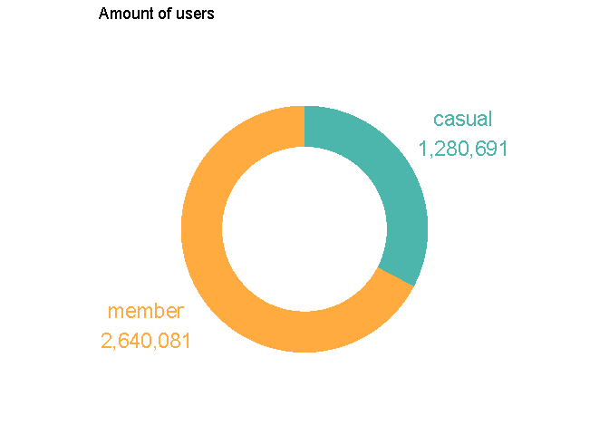 Amount of users
Descriptive analysis of the ride_length variable will provide insights and the distribution of ride duration across different user types.
summary(annual_data_v2$ride_length)

##    Min. 1st Qu.  Median    Mean 3rd Qu.    Max.
##   1.017   5.567   9.267  11.373  15.267  35.583

annual_data_v2 %>%
  filter(user_type == "member") %>%
  pull(ride_length) %>%
  summary()

##    Min. 1st Qu.  Median    Mean 3rd Qu.    Max.
##   1.017   5.133   8.500  10.546  13.967  35.583

annual_data_v2 %>%
  filter(user_type == "casual") %>%
  pull(ride_length) %>%
  summary()

##    Min. 1st Qu.  Median    Mean 3rd Qu.    Max.
##   1.017   6.733  11.050  13.080  17.917  35.583
Compare the two user types
aggregate(annual_data_v2$ride_length ~ annual_data_v2$user_type, FUN = mean)

##   annual_data_v2$user_type annual_data_v2$ride_length
## 1                   casual                   13.08008
## 2                   member                   10.54565

aggregate(annual_data_v2$ride_length ~ annual_data_v2$user_type, FUN = median)

##   annual_data_v2$user_type annual_data_v2$ride_length
## 1                   casual                      11.05
## 2                   member                       8.50

aggregate(annual_data_v2$ride_length ~ annual_data_v2$user_type, FUN = max)

##   annual_data_v2$user_type annual_data_v2$ride_length
## 1                   casual                   35.58333
## 2                   member                   35.58333

aggregate(annual_data_v2$ride_length ~ annual_data_v2$user_type, FUN = min)

##   annual_data_v2$user_type annual_data_v2$ride_length
## 1                   casual                   1.016667
## 2                   member                   1.016667
Convert to ordered factor the column and save the file for further analysis.
annual_data_v2$day_of_week <- ordered(annual_data_v2$day_of_week, levels=c("Monday", "Tuesday", "Wednesday", "Thursday", "Friday", "Saturday","Sunday"))
annual_data_v2$month <- ordered(annual_data_v2$month, levels=c("January", "February", "March", "April", "May", "June", "July", "August", "September", "October", "November", "December"))

write_csv(annual_data_v2, "D:/Proyecto_R/annual_data_v2.csv")
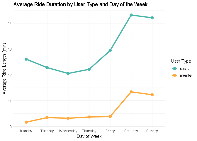
It can be observed that the duration of rides is longer for casual users during weekends.
annual_data_v2 %>%
  aggregate(ride_length ~ user_type + day_of_week, FUN = mean) %>%
  ggplot(aes(x = day_of_week, y = ride_length, color = user_type, group = user_type)) +
  geom_line(linewidth = 1.5) +
  geom_point(size = 3) +
  labs(title = "Average Ride Duration by User Type and Day of the Week", x = "Day of Week", y = "Average Ride Length (min)", color = "User Type") +
  scale_color_manual(values = c("casual" = "#4DB6AC", "member" = "#FFAB40")) +
  theme_minimal()
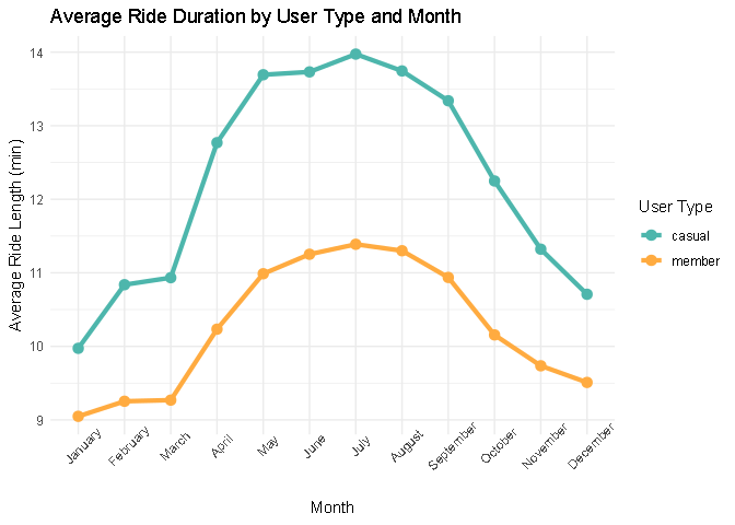
This chart allows for easy visualization of how the average ride duration varies between casual users and members throughout the months of the year.
annual_data_v2 %>%
  aggregate(ride_length ~ user_type + month, FUN = mean) %>%
  ggplot(aes(x = month, y = ride_length, color = user_type, group = user_type)) +
  geom_line(linewidth = 1.5) +
  geom_point(size = 3) +
  labs(title = "Average Ride Duration by User Type and Month"
  , x = "Month", y = "Average Ride Length (min)", color = "User Type") +
  scale_color_manual(values = c("casual" = "#4DB6AC", "member" = "#FFAB40")) +
  theme_minimal() +
  theme(axis.text.x = element_text(angle = 45))
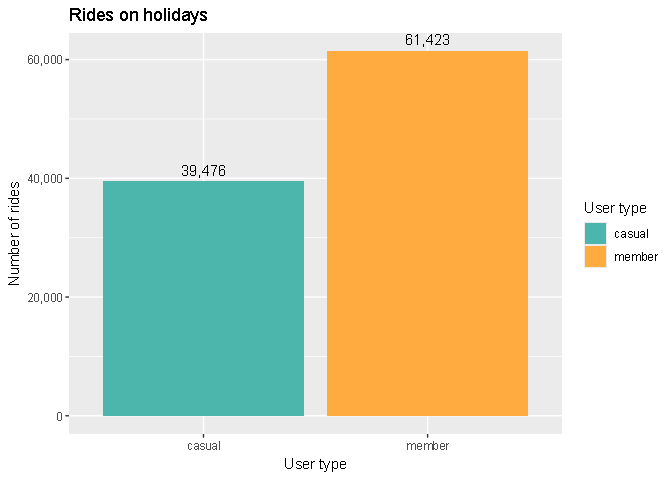
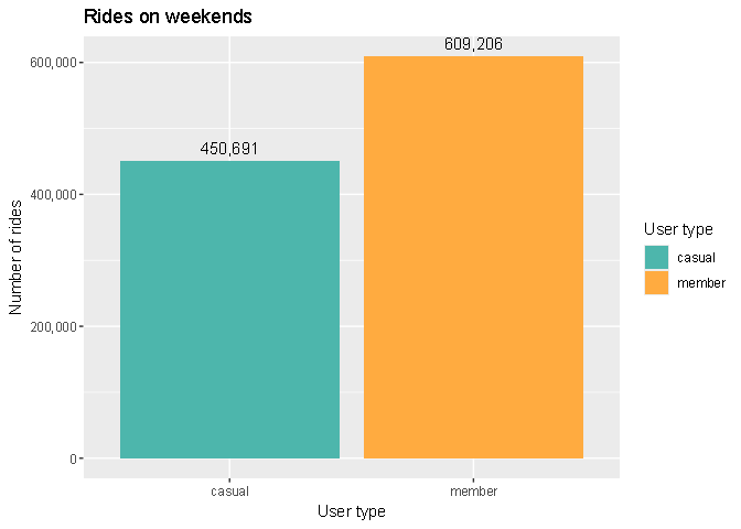
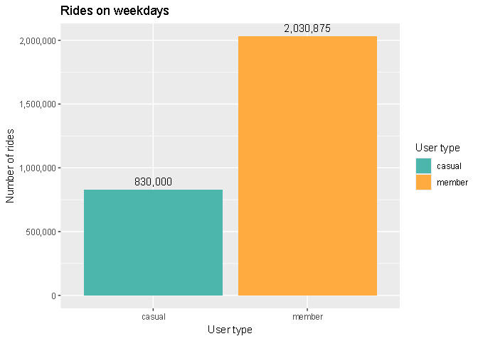
Analyze users data by user type, weekday, weekends and holidays. The number of rides on federal holidays is calculated using the cal_us_federal() function, which serves as an example calendar representing the federal holidays in the United States. This calendar is not historically accurate but reflects the currently recognized federal holidays.
holidays_2023 <- cal_events(cal_us_federal(), year = 2023)
annual_data_v2 %>%
  group_by(user_type) %>%
  inner_join(holidays_2023, by="date") %>%
  summarise(number_of_rides = n()) %>%
  ggplot(aes(x = user_type, y = number_of_rides, fill = user_type)) +
  scale_fill_manual(values = c("casual" = "#4DB6AC", "member" = "#FFAB40")) +
  geom_col(position = "dodge") +
  geom_text(aes(label = comma(number_of_rides)),
            position = position_dodge(width = 0.9),
            vjust = -0.5)+
  labs(title = "Rides on holidays", x = "User type", y="Number of rides", fill = "User type")  +
  scale_y_continuous(labels = comma)
annual_data_v2 %>%
  filter(day_of_week %in% c("Saturday", "Sunday")) %>%
  group_by(user_type) %>%
  summarise(number_of_rides = n()) %>%
  ggplot(aes(x = user_type, y = number_of_rides, fill = user_type)) +
  scale_fill_manual(values = c("casual" = "#4DB6AC", "member" = "#FFAB40")) +
  geom_col(position = "dodge") +
  geom_text(aes(label = comma(number_of_rides)),
            position = position_dodge(width = 0.9),
            vjust = -0.5)+
  labs(title = "Rides on weekends", x = "User type", y="Number of rides", fill = "User type")  +
  scale_y_continuous(labels = comma)
annual_data_v2 %>%
  filter(day_of_week %in% c("Monday", "Tuesday", "Wednesday", "Thursday", "Friday")) %>%
  group_by(user_type) %>%
  summarise(number_of_rides = n()) %>%
  ggplot(aes(x = user_type, y = number_of_rides, fill = user_type)) +
  scale_fill_manual(values = c("casual" = "#4DB6AC", "member" = "#FFAB40")) +
  geom_col(position = "dodge") +
  geom_text(aes(label = comma(number_of_rides)),
            position = position_dodge(width = 0.9),
            vjust = -0.5)+
  labs(title = "Rides on weekdays", x = "User type", y="Number of rides", fill = "User type")  +
  scale_y_continuous(labels = comma)
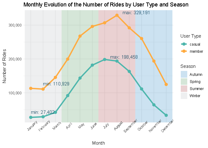
This creates a seasons data frame with columns representing the start and end months for each season, the name of each season, and a custom color for each. These values will be used later to mark the different seasons on the plot.
#data frame for later use in the plot
seasons <- data.frame(
  start = c(1, 4, 7, 10),  # Start month for each season
  end = c(3, 6, 9, 12),    # End month for each season
  season = c("Winter", "Spring", "Summer", "Autumn"),
  color = c("#0071bc", "#2e8540", "#981b1e", "#aeb0b5")  #color for each season
)
These two blocks of code find the months with the maximum and minimum number of rides for each user_type. The max_points and min_points data frames store these extreme values, which will later be used to add text annotations to the plot.
# Find the maximum points
max_points <- annual_data_v2 %>%
  group_by(user_type, month) %>%
  summarise(number_of_rides = n()) %>%
  filter(number_of_rides == max(number_of_rides))
# Find the minimum points
min_points <- annual_data_v2 %>%
  group_by(user_type, month) %>%
  summarise(number_of_rides = n()) %>%
  filter(number_of_rides == min(number_of_rides))
This code creates a comprehensive plot, comparing the monthly number of rides for casual and member users, with annotations for seasonal changes and the maximum and minimum values.
annual_data_v2 %>%
  mutate(weekday = wday(started_at, label = TRUE, week_start = 1, locale = "LC_TIME")) %>%
  group_by(user_type, month) %>%
  summarise(number_of_rides = n()) %>%
  arrange(user_type, month) %>%
  #plot
  ggplot(aes(x = month, y = number_of_rides, color = user_type, group = user_type)) +
  geom_rect(data = seasons, aes(xmin = start - 0.5, xmax = end + 0.5, ymin = -Inf, ymax = Inf, fill = season), inherit.aes = FALSE, alpha = 0.2) +
  geom_line(size = 1.5) +
  geom_point(size = 3) +
  geom_text(data = max_points, aes(label = paste("max:", comma(number_of_rides))), vjust = -.28, hjust = -.2, color = "#08415c") +
  geom_text(data = min_points, aes(label = paste("min:", comma(number_of_rides))), vjust = -1, hjust = 0, color = "#08415c") +
  scale_fill_manual(values = seasons$color) +
  labs(title = "Monthly Evolution of the Number of Rides by User Type and Season",
       x = "Month", y = "Number of Rides", color = "User Type", fill = "Season") +
  scale_color_manual(values = c("casual" = "#4DB6AC", "member" = "#FFAB40")) +
  scale_y_continuous(labels = comma) +
  theme_minimal() +
  theme(panel.background = element_rect(fill = NA, color = NA)) +
  theme(axis.text.x = element_text(angle = 45))
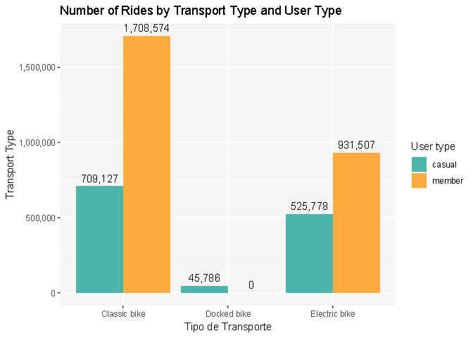
annual_data_v2 %>%
  group_by(user_type, rideable_type) %>%
  summarise(number_of_rides = n(), .groups = 'drop') %>%
  complete(user_type, rideable_type, fill = list(number_of_rides = 0)) %>%
  #plot
  ggplot(aes(x = rideable_type, y = number_of_rides, fill = user_type)) +
  scale_fill_manual(values = c("casual" = "#4DB6AC", "member" = "#FFAB40")) +
  geom_col(position = "dodge") +
  geom_text(aes(label = comma(number_of_rides)),
            position = position_dodge(width = 0.9),
            vjust = -0.5) +
  labs(title = "Number of Rides by Transport Type and User Type",
       x = "Transport Type",
       y = "Number of Rides", fill = "User type") +
  scale_x_discrete(labels=c("Classic bike", "Docked bike", "Electric bike"))+
  scale_y_continuous(labels = comma) +
  theme(panel.background = element_rect(fill = "#F5F5F5"))
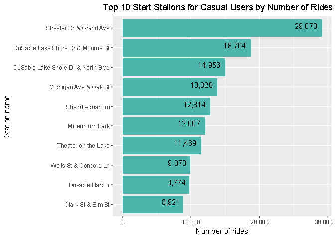
annual_data_v2 %>%
  filter(user_type == "casual") %>%
  group_by(start_station_name) %>%
  summarise(number_of_rides = n())%>%
  arrange(desc(number_of_rides)) %>%
  slice_max(order_by=number_of_rides,n = 10) %>%
  ggplot(aes(x=reorder(start_station_name, number_of_rides), y=number_of_rides))+
  labs(title="Top 10 Start Stations for Casual Users by Number of Rides", x="Station name", y = "Number of rides")+
  geom_bar(stat = "identity",fill = "#4DB6AC") +
  geom_text(aes(label = comma(number_of_rides)), hjust=1.2, vjust=.1) +
  scale_y_continuous(labels = comma)+
  coord_flip()
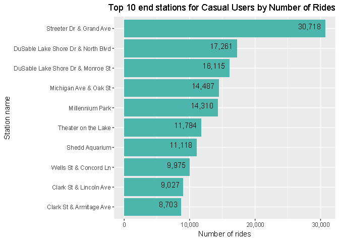
annual_data_v2 %>%
  filter(user_type == "casual") %>%
  group_by(end_station_name) %>%
  summarise(number_of_rides = n())%>%
  arrange(desc(number_of_rides)) %>%
  slice_max(order_by=number_of_rides,n = 10) %>%
  ggplot(aes(x=reorder(end_station_name, number_of_rides), y=number_of_rides))+
  labs(title="Top 10 end stations for Casual Users by Number of Rides", x="Station name", y = "Number of rides")+
  geom_bar(stat = "identity",fill = "#4DB6AC") +
  geom_text(aes(label = comma(number_of_rides)), hjust=1.2, vjust=.1) +
  scale_y_continuous(labels = comma)+
  coord_flip()
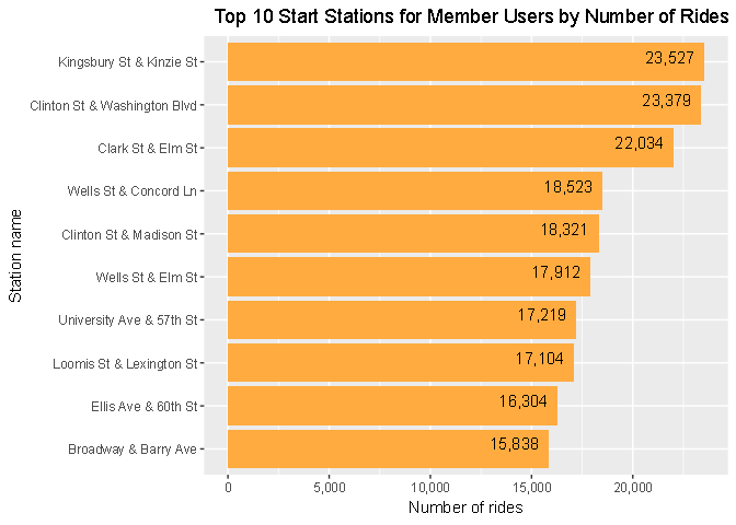
annual_data_v2 %>%
  filter(user_type == "member") %>%
  group_by(start_station_name) %>%
  summarise(number_of_rides = n())%>%
  arrange(desc(number_of_rides)) %>%
  slice_max(order_by=number_of_rides,n = 10) %>%
  ggplot(aes(x=reorder(start_station_name, number_of_rides), y=number_of_rides))+
  labs(title="Top 10 Start Stations for Member Users by Number of Rides", x="Station name", y = "Number of rides")+
  geom_bar(stat = "identity",fill = "#FFAB40") +
  geom_text(aes(label = comma(number_of_rides)), hjust=1.2, vjust=.1) +
  scale_y_continuous(labels = comma)+
  coord_flip()
annual_data_v2 %>%
  filter(user_type == "member") %>%
  group_by(end_station_name) %>%
  summarise(number_of_rides = n())%>%
  arrange(desc(number_of_rides)) %>%
  slice_max(order_by=number_of_rides,n = 10) %>%
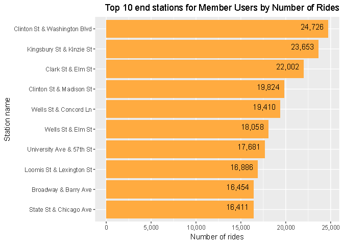
  ggplot(aes(x=reorder(end_station_name, number_of_rides), y=number_of_rides))+
  labs(title="Top 10 end stations for Member Users by Number of Rides", x="Station name", y = "Number of rides")+
  geom_bar(stat = "identity",fill = "#FFAB40") +
  geom_text(aes(label = comma(number_of_rides)), hjust=1.2, vjust=.1) +
  scale_y_continuous(labels = comma)+
  coord_flip()
Thank you so much for taking the time to check out my project!
References
-
Piasa, N. (2023, August 12). Google Data Analytics Capstone: Cyclistic Bike-Share (Python). Medium.
-
Data con Steven. (2024, January 3). Google Data Analytics | Proyecto Final | Caso Bellabeat [Video]. YouTube.